Introduction to Real time System & Real time Scheduling
 YUVRAJ HINGER
6 years ago | Programming paradigm
YUVRAJ HINGER
6 years ago | Programming paradigm

Share
Introduction
Real Time System, Types, Characteristics, Terms, Radar Signal Processing System, Periodic & Aperiodic task model, Real time Scheduling, Scheduling Criteria.
Table of Contents
- Part - I
- Real Time System –
- Types of real time systems supported timing constraints:
- Characteristics of Real-time Systems
- Difference between hard & soft real time system
- Terms related to real time system:
- Radar Signal Processing System
- Part - II
- Processor & Resource
- Parameter of Real time work load – Temporal, Functional & Resource
- Periodic & Aperiodic task model
- Real time Scheduling
- Scheduling Criteria
- Dynamic Versus Static System
- Effective Release time & deadline
- Off Line Versus On-Line Scheduling
- Part - III
- Clock Driven (offline/static schedulers)
- Timer-driven/Cyclic
- Priority Driven scheduling
- Fixed Priority Scheduling Algorithm
- Dynamic Priority-Driven Scheduling
- #. Schedulable test by RMA
Part - I
Real Time System –
sSoftware system where the proper functioning of the system depends on the results produced by the system with time at which these results are produced.
Example: flight control system, real time monitors etc.
Types of real time systems supported timing constraints:
1. Hard real time system –
- Can never miss its deadline.
- Missing the deadline may have disastrous consequences.
- The usefulness of result after deadline is completely 0.
- Example: Flight controller system.
2. Soft real time system –
- Can miss its deadline occasionally with some acceptably low probability.
- Missing the deadline have no disastrous consequences
- The usefulness of result after deadline is not completely 0 & consider as degraded service quality.
- Example: Telephone switches.
Characteristics of Real-time Systems
- Time Constraints, Correctness, Safety
- Concurrency, Stability, Embedded
Difference between hard & soft real time system
|
# |
Factor |
Hard vs soft |
|
1 |
Response time requirement |
less/high |
|
2 |
Timing constraints |
hard/soft |
|
3 |
Safety Critical |
true/false |
|
4 |
Database File Size |
small/large |
|
5 |
Deadline |
hard/soft |
|
6 |
Nature |
deterministic/non deterministic |
|
7 |
Accuracy |
high/low |
Terms related to real time system:
- Release time – time at which job becomes ready for execution
- Execution time – time taken by job to finish its execution
- Deadline – time by which a job should finish its execution.
- Absolute deadline = relative deadline + release time
- Relative deadline(d) = Maximum allowable response time
- Period – fixed time interval in which a particular task is being processed.
- Phase – release time of the first job in the periodic task.
- Lateness – Completion time - Deadline
- +ve Lateness is tardiness & -ve Lateness is earliness
- Tardiness – how late a real time system completes its task with respect to its deadline.
Radar Signal Processing System
1. Diagram

2. Working
Radar scans area by pointing its antenna in one direction at a time.
During scan it send short frequency pulse & examine the echo signal returning to antenna & determine whether there are objects(position & velocities) in the direction pointed by antenna.
The echo signal consist only background noise if there is no object.
The echo signal consist strong signal(examine strength & frequency) if there is any object.
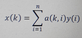
The digital sample value of echo signal is placed in buffer called bin & this are inputs to DSP & produce output using equation.
Equation –
Part - II
Processor & Resource
Processor – server & active resources carry out machine instruction, two processor are of same type if they have same function & used interchangeably. active component on which job is scheduled. ex – threads schedule on CPU, R/w request schedule on disk.
Resource – passive entity upon which jobs may depend. Usually reusable & not consumed by use. ex – memory.
Parameter of Real time work load – Temporal, Functional & Resource
Temporal Parameter –
describe timing constraints & behavioural of model.
Component
- Fixed Release time – release time exactly known.
- Jittered Release time – range of release time, not exactly known but within a range.
- Sporadic Release time – random release time, not known until the even trigger.
- Execution time
Functional Parameter
Component
- Preemption of jobs
- Criticality of jobs – urgency of job
- Optimal execution
- Laxity type & Laxity function – differentiate timing constraints (soft/hard). Usefulness of function is called laxity type of job.
Resource Parameter
Component
- Preemptivity of resources
- Resource graph – configuration of resource, relationship among resources.
Periodic & Aperiodic task model
Periodic – each computation or data transmission that is executed repeatedly at regular or semi-regular interval. Deterministic workload model.
Modelling
- Period = minimum length of all time intervals between release time of consecutive jobs.
- Execution time = max execution time of all jobs in this.
- Phase = release time of first job.
Aperiodic/Sporadic – set of job that execute at irregular time intervals. For soft deadline or no deadline. Ex- task to adjust radar’s sensitivity.
Real time Scheduling
Determine an feasible order of execution of tasks. A scheduler may be preemptive(control priority driven scheduling) or non-preemptive.
Classification of Real time Scheduling – Static & Dynamic Approach
1. Static Approach (Fixed-priority)
Priorities are - computed offline, assigned to each task, & maintain unaltered lifetime of task & system.
Required - complete prior knowledge of real time environment in which it is developed & little runtime overhead.
Inflexible scheduling
Work only for relatively simple systems.
2. Dynamic Approach
Priorities are - computed offline, assigned to each task, & can change at runtime as It schedule task dynamically upon arrival depend on task characteristics & current state of system.
Classification of Real time Scheduling Algorithm
1. Clock Driven (offline/static schedulers)
2. Hybrid Schedulers
- Scheduling decision at both clock interrupt points & event occurrence.
Popular Scheduler – Time-Sliced round robin scheduling
Weighted round robin scheduling – builds on the basic of round robin scheduling scheme, difference is giving different time shares to the jobs according to their weight. A job with weight wt gets wt time-slice every round.
3. Event Driven
- Scheduling decision by task arrival & its completion events.
- Handle aperiodic & sporadic tasks.
- Less efficient as they deploy more complex algorithm.
- Less suitable for embedded application
- Example of event scheduler – Foreground-Background, EDF & RMA scheduler.
Scheduling Criteria
- CPU utilization – max
- Throughput – no of processes completed per time unit
- Turnaround time – execution time + waiting time
- Waiting time – time in ready queue for process
- Response time – time for submission to the time for response produced.
- Covering reliability, security & safety
Dynamic Versus Static System
Dynamic System – ready jobs are placed in queue common to all processor. when a processor is available, job that head of execute on processor.
Static System – partition of job in system into subsystem & assign & bind subsystem statically to processor.
Effective Release time & deadline
Effective Release time – without predecessors = release time & with predecessors = max release time & effective release time of its predecessors.
Effective Deadline – without successor = deadline & with successor = min deadline & effective deadline of its successor.
Off Line Versus On-Line Scheduling
Off Line (clock driven) – Schedule is computed before system begins to execute & computation is based on knowledge of release time & processor time of all jobs. Disadvantage: Inflexibility
On-Line (priority driven) – Schedule without knowledge of jobs that will released in future or the parameter of job is known to schedular after job is released. Future work load is unpredictable.
Part - III
Clock Driven (offline/static schedulers)
- Used in hard real time system
- All parameter are fixed and known
- Schedule before system start to run
- Simple & efficient
- Used in embedded application
- Scheduling decision at the clock interrupt points.
- Little run time overhead & cannot handle aperiodic & sporadic tasks.
Features: table-driven & cycle schedulers
Table-driven – at time of system design, schedule task & store in table.
Timer-driven/Cyclic
– repeats a precomputed value. ex- temperature controller.
General Structure
1. Frame & Major Cycles
Partition time into intervals called frames. Every frame has length f (frame size).
Every scheduling decision are made only at beginning of frame, no Preemption within frame.
2. Frame Size Constraints
Helps to decide frame size.
Minimum context switching – every job can start & execute within frame,
f>=max (ei)
Frame Size – to keep length of cyclic schedule short, f should be chosen so that it divides H(hyper period length)
Rounddown(pi/f) - pi/f = 0
3. Job Slice
When task not meet frame size constraints then execution of each job by time slice.
Priority Driven scheduling
greedy(make locally optimal decision), list(assign priority) & work conversing scheduling. Job of task processed according to priority(urgency of job).
Preemptive, Non Preemptive Scheduling.
Fixed Priority Scheduling Algorithm
Assign same priority to all job.
1. RMA (Rate monotonic algorithm)
Priorities are assigned according to their period(shorter have higher priority). tasks are independent & no precedence constraints.
Schedulability test for RMA
Necessary condition:
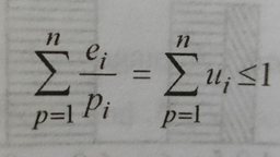
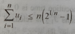
ei is worst case execution time, pi is period of task & n is total number of task.
Sufficient condition
2. DMA (Deadline monotonic algorithm)
Priorities are assigned according to their relative deadlines(shorter have higher priority).
RM & DM - When, Di=Pi Both are identical, Di<=Pi, DM is better to use
*when system is unschedulable with dm then it is unschedulable for all other.
Dynamic Priority-Driven Scheduling
Priority of tasks changes as other task released.
1. EDF (Earliest Deadline First) Algorithm
Priorities are assigned according to their absolute deadlines(shorter have higher priority).
2. LST (Least Slack Time) Algorithm
Priorities are assigned according to slack time(shorter have higher priority).
LST is job-level dynamic-priority & EDF is job-level fixed-priority algorithm.
At time t Slack of job = d(deadline) – t – x(exec time)
#. Schedulable test by RMA
Ti(p,e) - Test T1(10,2) T2(15,5) T3(25,9) schedulable by RMA
Necessary condition = 2/10 + 5/15 + 9/25 = 0.893 <=1
Sufficient condition = 3[2^(1/3)-1] = 0.779
0.893<=0.779 not satisfied, so not schedulable by RMA